At a glance
What this page covers
- For
- Power-electronics engineers defining labels, records, or datasets before training a model.
- You will leave with
- A four-part label contract that separates rule outcome, execution state, review requirement, and final disposition.
- Evidence status
- Published Field Note backed by a rebuildable simulation-only campaign at one frozen operating point.
- Boundary
- The campaign uses a simplified single-point equivalent model; it is not hardware approval, multi-point validation, or proof of solver equivalence.
Starting point, decision and reusable output
- Decision
- Decide whether a candidate record supports proceed, rework, review, or abstention without confusing software execution with electrical evidence.
- Starting point
- No machine-learning code is required; basic familiarity with LLC screening and engineering review is useful.
- Reusable output
- A 20-candidate Quickstart, a versioned 200-candidate evidence archive, and a replayable candidate record.
Run the beginner grouped-baseline lab, then compare its split and label contract with this LLC evidence loop.
A surrogate model does not learn engineering intent. It learns the relationships encoded in the records it receives. If pass sometimes means “the calculation ran”, sometimes “the analytical gate passed”, and sometimes “the design is acceptable”, adding more designs only scales the ambiguity. Before asking how much data a surrogate needs, the workflow must define exactly what each label means and preserve the evidence behind it.
This Field Note opens a series on building surrogate models for power-electronics design. Part one establishes that foundation by separating rule outcome, execution state, review requirement, and final disposition inside a replayable LLC workflow. A rule can pass or reject. An execution can complete or fail. A case can require review. A final decision can proceed, rework, abstain, or escalate.
To see why these distinctions matter, imagine reviewing 200 LLC candidates in a spreadsheet. For each one, you check required gain, input phase, solver completion, electrical limits, and the reason it did or did not advance. Now ask a coding assistant to automate that work. The calculations are not the hardest part. The hard part is preventing the software from calling a timeout a bad converter or writing PASS without saying what passed. This first step makes every later dataset decision interpretable: define the decision contract, run a small rebuildable demo, inspect every output, and keep the engineering meaning attached to each record.
With that foundation in place, the next Field Note will examine how far the design population must diversify before the records begin to support a useful surrogate, rather than merely describe one generator, one model, and one operating point.
Why “screen these designs” is not an engineering specification
An LLC screening request leaves critical decisions undefined:
- Which topology, equations, and operating condition are in scope?
- What does the first-harmonic approximation, or FHA, need to prove?
- Which quantities are measurements, calculated values, or model proxies?
- What happens when a numerical method does not finish?
- Does an automatic pass mean “advance to the next check” or “approve hardware”?
A coding assistant can fill those gaps with reasonable-looking assumptions. That is exactly the risk. Hidden assumptions become repeated decisions as soon as the workflow scales.
For a future surrogate, those repeated decisions become the target it tries to learn. A model can score well against an internally consistent table while learning the wrong engineering distinction. The purpose of this first Field Note is therefore not to train the surrogate. It is to make the future training records mean one consistent thing.
Current baseline: staged engineering review before automation
The manual baseline is a staged review. Freeze the specification and candidate bounds, inspect the FHA gain and input phase, send only eligible candidates to the next method, and record electrical rejections separately from methods that did not complete.
The bounded decision is whether a generated candidate:
- is rejected at the FHA gate;
- advances to a time-stepped linear-equivalent evaluation;
- passes or fails the named automatic electrical checks;
- is withheld because execution failed.
Hardware approval is outside that decision.
How one ambiguous label can corrupt the evidence set
Suppose the simulation software reaches a timeout. The converter may be poor, the numerical setup may be difficult, the model may be incomplete, or the allowed run time may simply be too short. None of those possibilities is an electrical rejection.
If the workflow stores that case as reject, later analysis sees a false physical label. If the same records are used for machine learning, the model learns simulation behaviour as though it were converter behaviour. A larger dataset then reinforces the mistake: the surrogate becomes better at reproducing the workflow's labelling error, not at recognising an electrically unacceptable LLC design.
The opposite error is just as serious. If a candidate passes a simplified single-point model and the report shows only PASS, the reader may interpret a screening result as a validated design.
Separate rule outcome, execution state, review, and final disposition
The workflow uses four distinct questions:
- Did the method complete, and did it converge where required?
- Did the named rule pass or reject the available result?
- Does the case require engineering review?
- What final disposition is authorised: proceed, rework, abstain, or escalate?
Those answers are stored separately. A failed execution has no electrical rule outcome. A rule can pass while the case still requires review. Review does not overwrite the evidence already recorded, and the final disposition states only the next action authorised from that evidence.
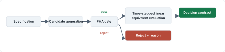
This separation is the core design choice. It keeps the software useful without giving it authority the evidence has not earned.
Build the evidence loop before adding model complexity
1. Freeze the electrical scope
The archived campaign used one half-bridge LLC operating condition with a centre-tapped secondary:
| Quantity | Frozen value |
|---|---|
| Input voltage | 400 V |
| Output voltage | 36 V |
| Output power | 230 W |
| Operating condition | Fixed input, full load |
| FHA frequency search | 50 to 180 kHz |
| Maximum FHA gain error | 1% |
| Minimum inductive input phase | 2° |
The scope label Phase A means preliminary electrical screening at this one operating point. It is an internal label, not an industry-standard design phase.
Magnetic design, semiconductor losses, thermal behaviour, EMI, control robustness, tolerances, line and load sweeps, and hardware validation are excluded. Naming those exclusions prevents a successful run from implying that they were checked.
2. Generate candidates deterministically
The frozen campaign generated 200 candidates with a deterministic Latin-hypercube process and seed 20260820. It varied resonant frequency, inductance ratio, quality factor, and transformer turns ratio.
Determinism matters because a reviewer can regenerate the same population and compare its content hash. Without a frozen seed, bounds, definitions, and configuration, a repeated run may test a different problem.
3. Use FHA as a fast analytical gate
For each candidate, the FHA stage searched the allowed frequency range. A candidate advanced only when it could reach the required gain within 1% while retaining at least 2° of inductive input phase.
FHA answers a bounded screening question. It does not reproduce every switching, nonlinear, magnetic, parasitic, or control effect.
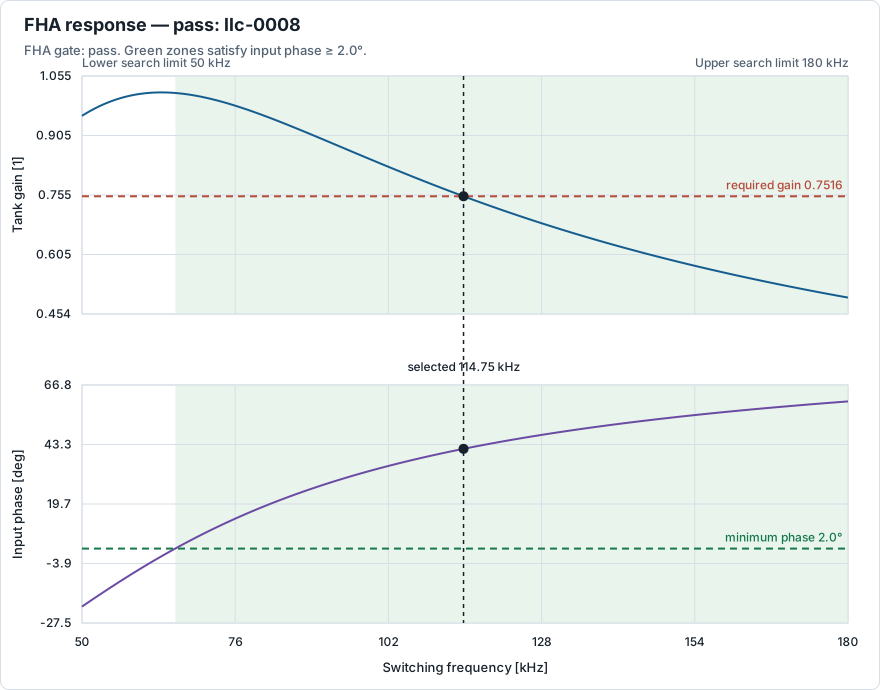
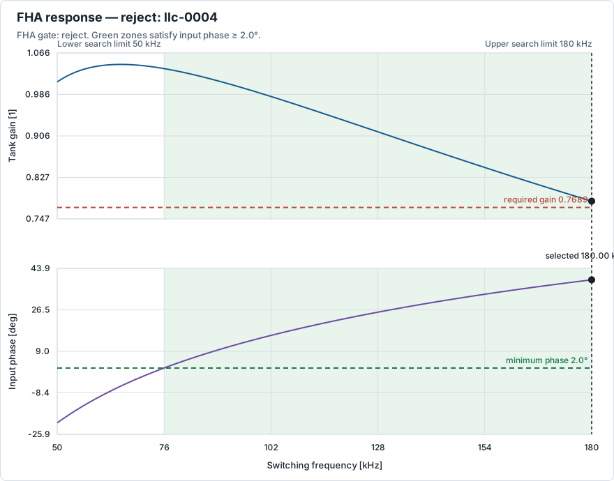
The plots make the decision inspectable. A pass shows the selected point, required gain, gain response, and input phase. A reject shows why the allowed region did not contain an acceptable point.
4. Evaluate survivors with the primary time-stepped method
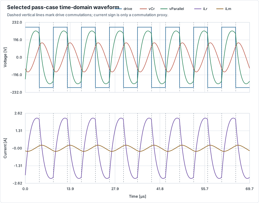
FHA survivors entered switched-linear-equivalent-v1, a time-stepped linear-equivalent model with explicit convergence and measurement windows. The archived campaign performed 168 of these evaluations.
The model adds time-domain evidence while remaining a simplified electrical representation. Its commutation-current signs are proxies inside that model, not proof of zero-voltage switching in a physical converter.
5. Write one record per candidate
Each record keeps the input specification and hash, candidate variables and units, methods, thresholds, convergence evidence, telemetry, decision reason, and provenance. Missing targets remain missing instead of receiving invented values.
The record also retains a human boundary: requires engineer review remains true and reviewed by remains empty until an authorised review occurs.
What the campaign can actually prove
The 200-candidate result
The verifier recovered all 200 records, checked the controlled status vocabulary, validated stored hashes, and reproduced the frozen candidate-set hash.
| Gate outcome | Count |
|---|---|
| Generated | 200 |
| FHA reject | 32 |
| FHA pass | 168 |
| Time-stepped linear-equivalent evaluations | 168 |
| Evaluation executions completed | 168 |
| Evaluation executions failed | 0 |
| Automatic rule pass | 168 |
| Automatic rule reject | 32 |
| Cases requiring engineering review | 200 |
| Engineer-authorised final dispositions | 0 |
All 32 analytical rejections used the archived reason FHA_GAIN_TARGET_NOT_REACHED. Their FHA rule outcome was reject, so they did not enter the more expensive primary method.
All 168 FHA survivors completed and converged in the time-stepped linear-equivalent method. Their named electrical rule outcome was pass at the frozen single point. It does not mean that 168 hardware designs were approved.
Five survivors selected the 180 kHz upper edge of the FHA search. The rebuildable schema marks that boundary condition so an edge optimum is not mistaken for a comfortably contained solution.
The current population also contains no FHA-versus-primary-method disagreement. That absence is not proof that the two methods are equivalent.
The notebook makes the small run visible
The downloadable notebook runs a new 20-candidate demonstration. It does not read the archived 200-candidate records.
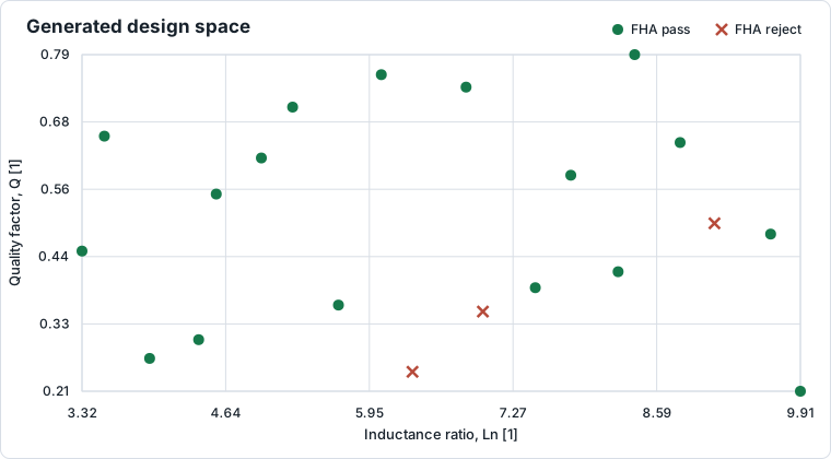
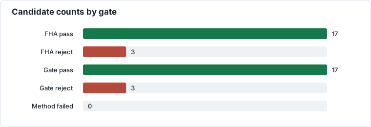
This small run is useful because the engineer can change the visible input values, run the workflow, and inspect the records and plots within one session. It demonstrates the bookkeeping and decision semantics without asking the reader to audit 200 cases first.
One recoverable candidate
Candidate llc-0186 was selected by the frozen ranking rule as the reusable record from the archived campaign.
| Design variable | Value |
|---|---|
| Resonant frequency | 72.999 kHz |
| Inductance ratio | 3.6118 |
| Quality factor | 0.6576 |
| Turns ratio, primary to secondary | 4.2289 |
| Resonant inductance | 117.103 µH |
| Magnetising inductance | 422.951 µH |
| Resonant capacitance | 40.592 nF |
The FHA gate selected 114.25 kHz. At that point, the gain error was 0.0127% and the calculated input phase was 42.68°, so the candidate advanced.
The time-stepped method converged after 90 cycles. Its eight-cycle, 1,280-sample measurement window produced:
| Telemetry | Value |
|---|---|
| Output voltage | 35.9767 V |
| Output power | 229.702 W |
| Equivalent-model power ratio | 95.3188% |
| Switching frequency | 114.25 kHz |
| Resonant-current peak | 2.347 A |
| Resonant-current RMS | 1.755 A |
| Magnetising-current peak | 0.669 A |
| Resonant-capacitor peak voltage | 86.268 V |
Its automatic rule outcome is pass. The case still requires engineering review, and no engineer-authorised final disposition is recorded. The result belongs to the frozen model, condition, and thresholds.
Replaying one candidate record
The campaign replayed llc-0186 in a separate evidence directory using the same configuration and method. The retained 1,280-sample waveform and every decision-relevant telemetry value matched the original record on the archived environment. The observed numerical delta was 0.0 for each compared metric.
Exact hashes establish archived integrity. Named numerical tolerances support cross-environment reproduction. Replay proves that the result can be reconstructed, not that the model is physically complete.
The simulation software timeout that must not become an electrical reject
A separate simulation software preflight exceeded its configured 180-second timeout and did not produce the required measurements.
Its execution status is failed, with reason SOLVER_TIMEOUT.
It is not reject.
The failed method produced no decision-safe electrical conclusion. It was archived outside the completed 200-candidate primary-method population and did not contaminate those labels.
The public archive retains a sanitized failure record and note.
This failure also blocks a stronger claim: the campaign has not established equivalence between the linear-equivalent primary method and a higher-fidelity closed-loop implementation.
Why these 200 records are not yet a trustworthy training dataset
All final decisions come from one fixed input and full-load condition. The evidence does not cover line, load, temperature, tolerances, magnetics, semiconductor stress, cross-solver validation, hardware correlation, or held-out design-level model evaluation.
The 168 passes are also one-sided after the FHA gate. A surrogate trained on these records could learn the boundaries of this generator and model while appearing more general than it is.
The next dataset should add controlled diversity and stronger cross-method evidence, not merely more rows.
This is where the next Field Note begins. It will ask how far that diversity must expand before an unseen-design evaluation becomes meaningful, and how to tell whether new candidates add coverage or only add density inside the same narrow region.
Run the files in the route that fits you
Start with the 20-candidate Quickstart ↗. The 200-candidate evidence archive ↗ is for deeper audit.
Route A: Windows, no programming setup
- Download the Quickstart ZIP and extract it.
- Open the extracted folder.
- Double-click run_demo.bat.
- Wait for the run to finish.
- Open the new LLC_Demo_Runs folder beside the extracted package.
- Open summary.html in your browser.
- Confirm that the report says OUTPUT INTEGRITY: PASS.
- Review the separate FHA execution, FHA gate, time-domain execution, final automatic disposition, warnings, and engineering-approval status.
OUTPUT INTEGRITY: PASS means that the expected files and consistency checks passed. It does not approve any candidate for hardware.
Route B: PowerShell
Open PowerShell in the extracted Quickstart folder and run:
py -B run_demo.pyTo change the visible electrical specification and candidate count:
py -B run_demo.py --vin 400 --vout 36 --pout 230 --candidates 20The output appears in LLC_Demo_Runs beside the package. Each run receives its own folder so the generated evidence does not overwrite the source package.
Route C: Jupyter or Colab
For a local notebook, open notebooks/llc_quick_demo.ipynb. For a browser-only route, open the Colab notebook ↗.
- Find the marked parameter cell.
- Edit Vin, Vout, Pout, or candidate count.
- Choose Run all.
- Read the gate-count and design-space plots first.
- Inspect the pass and reject FHA cases.
- Review the retained time-domain traces and the status definitions.
- Download the generated files if you want to compare or audit the run later.
What each output is for
| Output | What to inspect |
|---|---|
| summary.html | Human-readable result, warnings, plots, and separated status fields |
| candidate_records.csv | One tabular row per candidate for quick filtering |
| candidate_records.jsonl | Complete machine-readable records, one JSON object per line |
| manifest.json | Run identity, files, and content hashes |
| verification.json | Machine-readable integrity result and checks |
| pedagogical_cases.json | Selected pass, reject, and failure examples for review |
| plots/ | Workflow, design space, gate counts, FHA cases, and retained traces |
| ml_dataset_v1.csv | Bounded export for later data work, not a qualified training set |
| feature_dictionary.json | Feature names, units, and meanings |
| target_dictionary.json | Target definitions and missing-value semantics |
| split_manifest.json | Design-level grouping contract for future model evaluation |
| dataset_card.md | Scope, provenance, exclusions, and safe-use notes |
Replay and verify
From the Quickstart or Evidence Archive root:
py -B -m llc_tool replay
py -B -m unittest discover -s tests -p "test_*.py" -v
py -B VERIFY_RELEASE.py
Replay reconstructs the named record under the published contract. The tests check implementation behaviour. The release verifier checks package integrity and evidence relationships. None of these commands is a substitute for higher-fidelity simulation or hardware review.
The defensible conclusion is deliberately narrow:
- Result: the frozen loop completed with 32 FHA rejections and 168 single-point linear-equivalent passes.
- Artifact: llc-0186 can be reconstructed and replayed with traceable evidence.
- Failure: the simulation software timeout remained a method failure and was never relabelled as an electrical rejection.
Use the Quickstart to inspect that distinction yourself. Then subscribe to Field Notes for the next step: measuring how much design diversity is needed before an unseen-design evaluation becomes meaningful.