Where AI Helps in Power Electronics: A Beginner's Map

AI can help an engineer search through many candidates, approximate a slow calculation, or notice a pattern in measurements. It does not know the physics of your converter unless that knowledge is built into the task and checked against evidence. The useful question is: which decision would improve if you could make a reliable estimate or flag an unfamiliar pattern?

First, what does “AI” mean here?

For this article, AI mainly means machine learning: a program learns a relationship from examples. An input might be current, switching frequency, geometry, or a waveform. The desired output might be loss in watts, temperature in °C, or a fault label. Think of one row of data as a familiar test record: the operating conditions, the design settings, and the result observed under those conditions. Many such records can reveal relationships that are awkward to write as one simple equation.

The engineer still chooses the question, the reference calculation or measurement, the acceptable error, and what to do when the answer is uncertain. A model that estimates temperature is answering a different question from one that identifies a possible fault; they require different examples and different checks.

This is different from asking a language assistant to explain a datasheet. A generated explanation can save reading time, but it must be checked against the original datasheet and the design conditions before it influences a component choice.

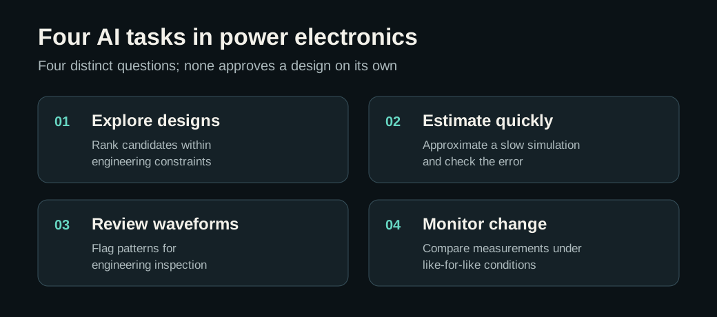
1. Explore design candidates

A converter design has competing targets: efficiency, ripple, temperature, volume, cost, and stress. AI can help rank candidates within constraints that the engineer defines. In one published study, researchers used simulation data, a neural model, and an optimization algorithm to select parameters for a 48 V to 12 V synchronous buck converter; they also reported hardware experiments for that specific case. This supports the possibility of assisted design, not an automatic approval process for other buck converters. Read the original study ↗.

A useful first question is small: “Which combinations of inductance and switching frequency are worth simulating in detail?” The output is a shortlist. Circuit simulation, thermal checks, tolerances, and prototype measurements still decide whether a candidate is acceptable.

Imagine a buck design with a specified input range, output voltage, and load range. Each candidate record could contain inductance, switching frequency, and a component choice. Its reference results could include ripple, estimated losses, and the hottest simulated operating point. A search method can then propose combinations that meet the stated limits and deserve a closer look. If no candidate meets the limits, that is useful information too: the constraints or available components may need revisiting.

The helpful output is a shortlist with reasons: which limit is close for each candidate, which operating points have been checked, and which simulations are still missing. The winner at nominal input and load may be a poor choice at minimum input, full load, startup, or high ambient temperature. Those conditions belong in the engineer's review before a design is selected.

2. Estimate a slow simulation result

A surrogate model learns to approximate an expensive simulation. For example, a researcher might simulate a set of heat-sink geometries, train a faster model to estimate a thermal result, then screen more geometries. A study of IGBT module heat sinks used a polynomial surrogate in place of repeated computational fluid dynamics runs during optimization and evaluated accuracy and uncertainty in that setting. Read the original heat-sink study ↗.

Here the input is a set of dimensions, materials, dissipated power, and cooling conditions; the target might be the maximum temperature returned by the detailed thermal simulation. The model can provide a quick estimate while exploring the same design region. The engineer can spend the slower simulations on candidates near a temperature limit, surprising predictions, and final choices. The reference simulations remain the source of truth for that task.

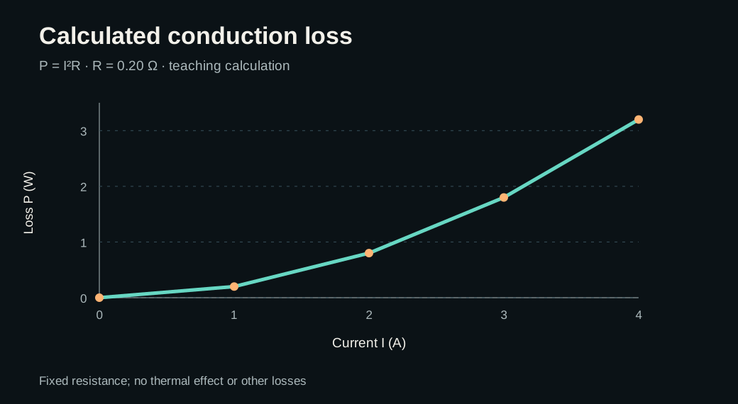
Before training anything, plot the simplest known relationship. This teaching example uses the conduction-loss equation P = I²R with a fixed resistance of 0.20 Ω. At 2 A it gives 0.8 W; at 4 A it gives 3.2 W. The curve is a calculation, not an AI prediction or a measured device result. Real resistance changes with temperature and the full converter has other losses.

If a model cannot improve a useful engineering baseline on unseen conditions, its extra complexity has not earned a place in the workflow.

An acceptance check should ask where the errors occur, not only how small their average is. Reserve complete geometries or device families for testing, and plot prediction minus simulation against power and geometry. A model that looks good in the middle of the design space but misses the hottest candidates is unsuitable for temperature-limit screening. Outside the range that has been tested, the workflow should request another simulation instead of returning a confident-looking number.

3. Review waveforms for possible faults

Current and voltage waveforms can contain patterns associated with operating changes or faults. A model can flag or classify a pattern for review. Research on IGBT open-circuit faults in three-phase inverters used phase currents and included offline and real-time experiments. The authors also explain why a model trained on one converter may not transfer cleanly to another with different parameters. Read the original fault-diagnosis study ↗.

The engineer should ask what was actually recorded: topology, load, input voltage, temperature, sampling rate, sensor position, and whether the example came from simulation or hardware. A “fault” label without that context is weak evidence. A flag should lead to a defined engineering check, not automatically to a repair or control action.

For a beginner's task, start with a narrow question such as whether a set of simulated phase-current traces looks like the defined normal cases. Keep the operating point attached to every trace. The output can be normal, review, or unfamiliar; an unfamiliar trace need not be forced into one of the known fault classes. This is useful when an engineer has many records to inspect, provided the review queue is small enough to use.

Evaluate the mistakes that matter. A false alarm costs investigation time; a missed fault can have a different consequence. Test complete runs or converter units that were kept out of training, then inspect the traces behind the mistakes. A change in sensor scaling, control mode, or load can resemble a fault to a model that has never seen it.

4. Monitor change over time

Repeated measurements can help reveal drift: for example, a temperature rise at comparable load and ambient conditions. AI may help distinguish a change worth investigating from normal variation. A study of photovoltaic inverters trained and tested a failure-prognosis model on field measurements that included operational and weather-related factors. That is evidence for the studied inverters; the time history, sensor quality, and actual failure labels determine whether a useful warning is possible elsewhere. Read the original field-measurement study ↗.

Suppose an inverter reports heatsink temperature each day. Comparing today's value with yesterday's is misleading if load and ambient temperature changed. A useful monitor compares similar conditions over time and records whether a change persists. It might produce a trend and a prompt to inspect cooling, sensors, or operating history. The first action is to check the observation and its context, because a sensor issue or a changed operating schedule can also produce a new pattern.

There is a large difference between saying “this behaviour deserves inspection” and predicting a remaining lifetime. The latter needs credible failure histories, a defined prediction horizon, and evaluation of missed and premature warnings. Start with the narrower monitoring question when those records are unavailable.

Two graphs, and what they do not prove

The next graph is another calculated teaching baseline. For an ideal buck converter with Vin = 24 V, Vout = 12 V, L = 100 µH and D = Vout/Vin = 0.5, the approximate inductor-current ripple is ΔI = (Vin − Vout)D/(L f). It falls from 1.2 A at 50 kHz to 0.3 A at 200 kHz. This deliberately leaves out switching loss, magnetic loss, control behaviour, parasitics, and component limits. It is useful for framing a question; it cannot select a frequency on its own.

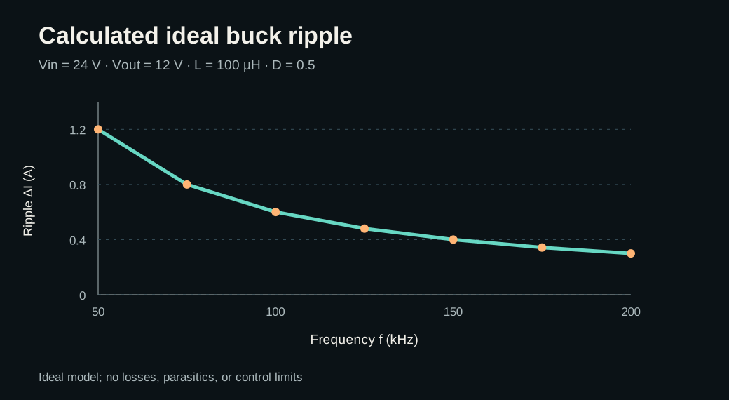
These graphs show why a model needs a reference. You can use equations where they apply, simulation for behaviour they omit, and measurement for the physical unit. A trained model is only an additional tool if it helps with the actual decision.

For example, lowering the calculated ripple by increasing switching frequency does not tell you what happened to switching loss or temperature. That missing trade-off is a plausible reason to gather simulation or measured data and test a model. The graph itself is the starting check: every proposed result should remain physically plausible alongside it.

A safe first experiment

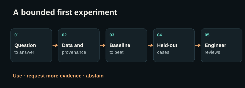
1. Choose one question. Example: estimate conduction loss across a specified current range, or flag one clearly defined simulated waveform pattern. Write down what decision the answer would change. A vague aim such as “use AI to improve the converter” is too broad to evaluate.
2. Name the reference. State whether the answer comes from an equation, a specific simulation model, or a measurement. Record units, operating conditions, and the source of each row. A simulated label and a measured label should remain distinguishable.
3. Build the simple baseline. Use the existing equation, a clear rule, or a straightforward interpolation. Plot its output first and note where it stops applying. This gives the model something meaningful to beat and exposes obvious data errors before training.
4. Hold back genuinely new cases. Test on conditions the model did not learn from. If several rows come from one converter, keep that converter together when splitting the data; for a time trend, reserve later observations. Official scikit-learn guidance ↗ explains why testing on training data exaggerates performance and why grouped or time-aware splits matter.
5. Inspect errors and choose an action. Plot errors against current, temperature, operating point, or device family. Check the worst relevant cases as well as the average. Define when to use the estimate, request a simulation or measurement, or stop. The final output of this experiment is that decision rule and the evidence behind it.